Question # 4
What does the "SQL keyword" refer to in the context of adding filters to a worksheet?
A.
The name of the function used to generate the filter
B.
The filter name to be inserted into queries
C.
The table name containing the static filter "key" values
D.
The name of a User-Defined Function (UDF) used to define the filter "key" values
Full Access
Answer:
B
Explanation:
In Snowsight (Snowflake's web interface), Data Analysts can create interactive dashboards and worksheets using Filters. When you define a filter (such as a Date Range or a list of Regions), you must assign it a SQL Keyword.
This "SQL Keyword" acts as a variable placeholder within your SQL code. For example, if you create a filter for "Customer Region" and set the SQL keyword to :my_region, you can then write a query like: SELECT * FROM sales WHERE region = :my_region. When a user interacts with the UI and selects "North America" from the dropdown, Snowsight automatically injects "North America" into every instance where :my_region appears in the worksheet's SQL.
Evaluating the Options:
Option A is incorrect because the keyword is a label/variable, not the underlying function code.
Option C and Option D are incorrect as they confuse the data source of the filter values with the reference name used in the SQL code.
Option B is the correct answer. The SQL Keyword is specifically the identifier (prefixed with a colon in the code) that allows the analyst to link the UI element (the filter) to the execution logic of the query. This is a fundamental skill for the Data Presentation and Data Visualization domain, ensuring reports are dynamic and user-friendly.
Question # 5
Consider the following chart.
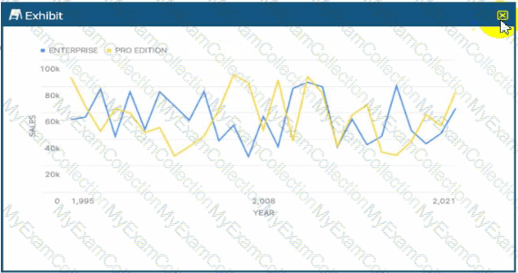
What can be said about the correlation for sales over time between the two categories?
A.
There is a positive correlation.
B.
There is a negative correlation.
C.
There is no correlation. (Selected)
D.
There is a non-linear correlation.
Full Access
Answer:
C
Explanation:
In Data Analysis, correlation refers to a statistical relationship between two variables. When analyzing a time-series chart like the one provided, a Data Analyst looks for patterns in how the two categories—"Enterprise" (blue line) and "Pro Edition" (yellow line)—move in relation to one another over the X-axis (Year).
A Positive Correlation would be indicated if both lines generally moved in the same direction at the same time (e.g., when Enterprise sales increase, Pro Edition sales also increase). A Negative Correlation (or inverse correlation) would be shown if the lines moved in opposite directions consistently (e.g., when one peaks, the other troughs).
Looking closely at the provided exhibit, the fluctuations for both editions are highly erratic and appear independent of each other. For instance, around the year 2008, the Pro Edition (yellow) shows a significant peak while the Enterprise edition (blue) experiences a sharp decline. Conversely, in other sections of the chart, they both dip or rise simultaneously by chance, but there is no sustained, predictable pattern of movement. The peaks and valleys do not align in a way that suggests one variable's movement is tied to the other.
Statistically, this lack of a discernible relationship indicates a Correlation Coefficient near zero. In the context of the Snowflake Snowpro Advanced: Data Analyst exam, identifying "No Correlation" is a key skill for interpreting Snowsight visualizations. It tells the analyst that the factors driving sales for the Enterprise tier are likely distinct from those driving the Pro Edition, and they should be analyzed as independent segments rather than interdependent variables. Therefore, based on the visual evidence of random, non-synchronous movement across the timeline, the only supported conclusion is that there is no correlation.
Question # 6
What functions should a Data Analyst use to run descriptive analytics on a data set? (Select TWO).
A.
REGR_INTERCEPT
B.
REGR_SLOPE
C.
ROW_NUMBER
D.
APPROX_COUNT_DISTINCT
E.
AVG
Full Access
Answer:
D, E
Explanation:
Descriptive analytics is the process of using historical data to understand "what happened." This typically involves summarizing large datasets into interpretable chunks using central tendency, dispersion, and frequency measures.
AVG (Average) is a cornerstone of descriptive statistics. It provides the arithmetic mean of a numeric column, allowing an analyst to understand the "typical" value within a dataset (e.g., Average Order Value).
APPROX_COUNT_DISTINCT is a descriptive tool used to understand the volume of unique entities within a dataset (e.g., "How many unique customers visited the site?"). Similar to HLL mentioned earlier, this function provides a fast summary of data volume and variety, which is a primary goal of the descriptive phase of analysis.
Evaluating the Options:
Options A and B (REGR_INTERCEPT and REGR_SLOPE) are used for linear regression. These fall under Predictive Analytics, as they are used to model relationships and predict future outcomes, rather than just describing current data.
Option C (ROW_NUMBER) is a window function used for data ranking and ordering, but it does not provide a descriptive summary of the dataset's characteristics.
Options D and E are correct because they provide summary statistics (mean and cardinality) that define the "state" of the data, which is the definition of descriptive analytics.
Question # 7
What scheme is used by Snowflake to estimate the approximate similarity between two or more data sets?
A.
MINHASH
B.
APPROX_PERCENTILE
C.
HyperLogLog
D.
APPROX_TOP_K
Full Access
Answer:
A
Explanation:
Snowflake provides several "approximate" functions designed to handle massive scale with high efficiency. While HyperLogLog (HLL) is the standard for estimating cardinality (unique counts), and APPROX_TOP_K is used for frequency estimation, the specific task of determining the similarity between two sets relies on a different probabilistic algorithm.
The MINHASH function is Snowflake's implementation for estimating the Jaccard similarity coefficient between two or more sets. Jaccard similarity is defined as the size of the intersection divided by the size of the union of the sample sets. Calculating an exact Jaccard similarity on billions of rows would be computationally expensive. MINHASH solves this by creating a "signature"—a small, fixed-size binary representation of the data. By comparing these signatures rather than the raw data, Snowflake can efficiently estimate how similar the original datasets are.
Evaluating the Options:
Option B (APPROX_PERCENTILE) is used to estimate the value at a specific percentile (e.g., the 95th percentile of latency).
Option C (HyperLogLog) is used for estimating cardinality (the number of unique elements), not the similarity between sets.
Option D (APPROX_TOP_K) identifies the most frequent elements in a dataset.
Option A is the 100% correct answer. It is the specific function built into Snowflake for similarity estimation using the MinHash scheme.
Question # 8
A Data Analyst is working with a table that has 1 record per day, with sales information. Which window function would calculate a 7-day moving average of sales, where SALES_DATE represents the date column?
A.
SUM(SALES) OVER (ORDER BY SALES_DATE ROWS BETWEEN 6 PRECEDING AND CURRENT ROW)
B.
SUM(SALES) OVER (ORDER BY SALES_DATE ROWS BETWEEN 7 PRECEDING AND CURRENT ROW)
C.
AVG(SALES) OVER (ORDER BY SALES_DATE ROWS BETWEEN 6 PRECEDING AND CURRENT ROW)
D.
AVG(SALES) OVER (ORDER BY SALES_DATE ROWS BETWEEN 7 PRECEDING AND CURRENT ROW)
Full Access
Answer:
C
Explanation:
Calculating a moving average (or rolling average) is a standard time-series analysis technique used to smooth out short-term fluctuations and highlight longer-term trends. In Snowflake, this is accomplished using Window Functions and the ROWS framing clause.
To calculate a 7-day moving average when you have one record per day, the "window" or "frame" must encompass exactly 7 rows. In SQL windowing syntax, the CURRENT ROW counts as one of those days. Therefore, to reach a total of 7, you need to look back at the 6 preceding rows ($6 + 1 = 7$).
Evaluating the Options:
Options A and B use the SUM() function. While the sum is part of an average, the question specifically asks for the average itself.
Option D is incorrect because 7 PRECEDING AND CURRENT ROW actually creates an 8-day window (the current day plus the seven days before it).
Option C is the 100% correct answer. It uses the AVG() aggregate function and correctly defines the frame as 6 PRECEDING AND CURRENT ROW, ensuring the calculation reflects exactly one week of data including the current day.
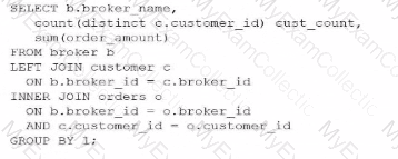
Question # 9
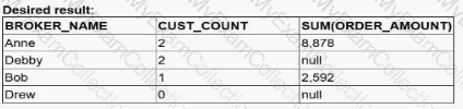
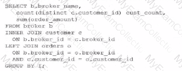
A Data Analyst is working with three tables:
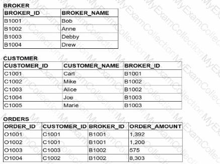
Which query would return a list of all brokers, a count of the customers each broker has. and the total order amount of their customers (as shown below)?
A)
B)
C)
D)
A.
Option A
B.
Option B
C.
Option C
D.
Option D
Full Access
Answer:
C
Explanation:
To achieve the desired result, an analyst must understand the fundamental behavior of different JOIN types within Snowflake and how they affect the retention of records from the "left" or primary table. The goal here is to list all brokers, even those who have zero customers (like "Drew") or customers with zero orders (like "Debby").
In SQL, an INNER JOIN only returns rows when there is a match in both tables. If we were to use an INNER JOIN between BROKER and CUSTOMER, Drew would be excluded from the results because he has no associated records in the CUSTOMER table. Similarly, an INNER JOIN with the ORDERS table would exclude any broker whose customers haven't placed an order.
Evaluating the Join Logic:
Option C is the correct solution because it utilizes a chain of LEFT JOINs. A LEFT JOIN (or LEFT OUTER JOIN) ensures that every record from the left table (BROKER) is preserved in the result set. If no matching record exists in the joined table (CUSTOMER or ORDERS), Snowflake populates the columns with NULL. This is why "Drew" appears with a CUST_COUNT of 0 and "Debby" appears with a NULL for the total order amount.
Option A fails because it uses an INNER JOIN for the CUSTOMER table, which would immediately filter out "Drew."
Option B and Option D fail because they use INNER JOINs at different stages of the query, which would strip away brokers or customers that do not have matching order activity.
Additionally, the query correctly uses COUNT(DISTINCT c.customer_id) to ensure that customers are not double-counted if they have multiple orders, and GROUP BY 1 (referencing b.broker_name) to aggregate the data at the broker level. This pattern is essential for accurate Data Analysis in Snowflake when dealing with "optional" relationships in a star or snowflake schema.
Question # 10
A Data Analyst has a very large table with columns that contain country and city names. Which query will provide a very quick estimate of the total number of different values of these two columns?
A.
SELECT DISTINCT COUNT(country, city) FROM TABLE1;
B.
SELECT HLL(country, city) FROM TABLE1;
C.
SELECT COUNT(DISTINCT country, city) FROM TABLE1;
D.
SELECT COUNT(country, city) FROM TABLE1;
Full Access
Answer:
B
Explanation:
When working with very large tables, calculating the exact number of unique combinations of columns (cardinality) using COUNT(DISTINCT ...) is a resource-intensive operation. It requires the Snowflake query engine to keep an exhaustive list of every unique pair encountered in memory, which can lead to high credit consumption and performance bottlenecks.
To provide a "very quick estimate," Snowflake utilizes the HyperLogLog (HLL) algorithm. The function HLL(column1, column2, ...) returns an HLL state (a binary representation) that can be used to estimate the number of distinct values with a high degree of accuracy and minimal computational overhead. This is part of Snowflake's suite of approximate aggregation functions, which are essential for Data Analysis on massive datasets where a 1% margin of error is acceptable in exchange for significantly faster results.
Evaluating the Options:
Option A is syntactically incorrect; DISTINCT cannot be used in that position with COUNT.
Option C is a valid query but will be significantly slower and more expensive than an HLL estimate on a "very large table".
Option D simply counts the total number of non-null rows, which does not represent the "number of different values" (cardinality).
Option B is the 100% correct answer. It specifically addresses the requirement for a "quick estimate" using the industry-standard probabilistic counting method built into Snowflake.
Question # 11
Which query will provide this data without incurring additional storage costs?
A.
CREATE TABLE DEV.PUBLIC.TRANS_HIST LIKE PROD.PUBLIC.TRANS_HIST;
B.
CREATE TABLE DEV.PUBLIC.TRANS_HIST AS (SELECT * FROM PROD.PUBLIC.TRANS_HIST);
C.
CREATE TABLE DEV.PUBLIC.TRANS_HIST CLONE PROD.PUBLIC.TRANS_HIST;
D.
CREATE TABLE DEV.PUBLIC.TRANS_HIST AS (SELECT * FROM PROD.PUBLIC.TRANS_HIST WHERE extract(year from (TRANS_DATE)) = 2019);
Full Access
Answer:
C
Explanation:
Snowflake utilizes a unique architecture known as Zero-Copy Cloning, which allows users to create a replica of a table, schema, or entire database without physically duplicating the underlying data files (micro-partitions). When you execute the CLONE command, Snowflake simply creates new metadata that points to the existing micro-partitions of the source object.
Because the data is not physically copied, the clone operation is nearly instantaneous and, crucially, incurs no additional storage costs at the moment of creation. Storage costs only begin to accumulate for the clone when the data in the source or the clone diverges—for example, if rows are updated or deleted in the clone, Snowflake creates new micro-partitions to store the changed data while preserving the original state in the source.
Evaluating the Options:
Option A (LIKE) only copies the column definitions and structure of the table. It does not copy the data itself, so while it doesn't incur storage, it also doesn't provide the "data" requested by the prompt.
Option B (CTAS - Create Table As Select) performs a full deep copy of the data. This creates entirely new micro-partitions, which immediately increases the storage footprint and associated costs.
Option D is a filtered CTAS operation. While it may result in less data than the full table, it still involves creating new physical storage for the 2019 records, thus incurring additional costs.
Option C is the 100% correct answer. It uses the CLONE keyword, which is the specific Snowflake feature designed to provide a full dataset for dev/test environments with zero initial storage impact. This is a core competency in the Data Transformation and Data Modeling domain.
Question # 12
Why would a Data Analyst use a dimensional model rather than a single flat table to meet BI requirements for a virtual warehouse? (Select TWO).
A.
Dimensional modelling will improve query performance over a single table.
B.
Dimensional modelling will save on storage space since it is denormalized.
C.
Combining facts and dimensions in a single flat table limits the scalability and flexibility.
D.
Dimensions and facts allow power users to run ad-hoc analyses.
E.
Snowflake generally performs better with dimensional modelling.
Full Access
Answer:
C, D
Explanation:
In the field of data warehousing and business intelligence (BI), choosing the right data model is crucial for long-term maintainability and user accessibility. While a single flat table might seem simple initially, dimensional modeling (typically using Star or Snowflake schemas) provides distinct advantages for enterprise analytics.
1. Scalability and Flexibility (Option C)
Combining all attributes into a single flat table creates a highly rigid structure. Every time a new attribute is added to a dimension (e.g., adding a "Promotion Category" to a product), the entire flat table must be rewritten or altered, which is inefficient for large datasets. Furthermore, flat tables often contain redundant data, leading to "update anomalies" where a change in a dimension attribute must be propagated across millions of rows. A dimensional model separates changing business processes (Facts) from the context of those processes (Dimensions), allowing the schema to scale and evolve independently.
2. Ad-hoc Analysis for Power Users (Option D)
Dimensional models are specifically designed to be intuitive for business users and BI tools. By organizing data into Facts (measurable metrics) and Dimensions (descriptive attributes), power users can easily "slice and dice" data across different hierarchies. For example, a user can quickly run an ad-hoc query to compare "Total Sales" (Fact) by "Store Region" (Dimension) and "Calendar Month" (Dimension). This structure provides a predictable and standardized "language" for the data, making it easier for users to build their own reports without needing a Data Analyst to create a custom flat table for every specific request.
Evaluating the Distractors:
Option A and E: These are common misconceptions. Modern cloud data warehouses like Snowflake are often highly optimized for wide "flat" tables due to columnar storage and sophisticated pruning. In many cases, a flat table may actually outperform a multi-table join (dimensional model) because it avoids the computational overhead of the join itself.
Option B: This is factually incorrect. Flat tables are denormalized (repeating data), which generally takes more storage space. Dimensional modeling is a form of normalization that saves space by storing descriptive strings once in a dimension table rather than repeating them for every transaction in a fact table.
Question # 13
When building a Snowsight dashboard that will allow users to filter data within a worksheet, which Snowflake system filters should be used?
A.
Include the :datebucket system filter in a WHERE clause, and include the :daterange system filter in a GROUP BY clause.
B.
Include the :daterange system filter in a SELECT clause, and include the :datebucket system filter in a GROUP BY clause.
C.
Include the :datebucket system filter in a WHERE clause, and include the :daterange system filter in a SELECT clause.
D.
Include the :daterange system filter in a WHERE clause, and include the :datebucket system filter in a GROUP BY clause.
Full Access
Answer:
D
Explanation:
Snowsight provides special System Keywords that allow analysts to create dynamic, interactive dashboards without hard-coding dates. Two of the most critical keywords are :daterange and :datebucket.
The :daterange keyword is designed to filter the volume of data based on a time period selected by the user in the dashboard UI (e.g., "Last 30 days" or "Current Year"). Because it acts as a filter on the underlying data, it must be placed in the WHERE clause of the SQL statement (e.g., WHERE created_at = :daterange). This ensures that only the records within the selected timeframe are processed by the query.
The :datebucket keyword is used for time-series aggregation. It allows the user to dynamically change the granularity of the data—for example, switching a chart from "Daily" to "Monthly" views without rewriting the query. To achieve this, :datebucket is used inside a date-truncation function in the SELECT list and, crucially, must be included in the GROUP BY clause to correctly aggregate the metrics (e.g., GROUP BY 1 or GROUP BY :datebucket).
Evaluating the Options:
Option A is incorrect because :datebucket is for grouping/truncation, not for filtering in a WHERE clause.
Option B is incorrect because :daterange is a filter (returning a range), not a scalar value suitable for a SELECT list.
Option C is incorrect for the same reasons as A and B.
Option D is the 100% correct answer. It follows the standard Snowsight design pattern: :daterange restricts the data rows in the WHERE clause, while :datebucket defines the temporal aggregation level in the GROUP BY clause.
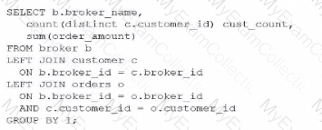
Question # 14
A Data Analyst is working with three tables:
Which query would return a list of all brokers, a count of the customers each broker has. and the total order amount of their customers (as shown below)?
A)
B)
C)
D)
A.
Option A
B.
Option B
C.
Option C
D.
Option D
Full Access
Answer:
C
Explanation:
To achieve the desired result, an analyst must understand the fundamental behavior of different JOIN types within Snowflake and how they affect the retention of records from the "left" or primary table. The goal here is to list all brokers, even those who have zero customers (like "Drew") or customers with zero orders (like "Debby").
In SQL, an INNER JOIN only returns rows when there is a match in both tables. If we were to use an INNER JOIN between BROKER and CUSTOMER, Drew would be excluded from the results because he has no associated records in the CUSTOMER table. Similarly, an INNER JOIN with the ORDERS table would exclude any broker whose customers haven't placed an order.
Evaluating the Join Logic:
Option C is the correct solution because it utilizes a chain of LEFT JOINs. A LEFT JOIN (or LEFT OUTER JOIN) ensures that every record from the left table (BROKER) is preserved in the result set. If no matching record exists in the joined table (CUSTOMER or ORDERS), Snowflake populates the columns with NULL. This is why "Drew" appears with a CUST_COUNT of 0 and "Debby" appears with a NULL for the total order amount.
Option A fails because it uses an INNER JOIN for the CUSTOMER table, which would immediately filter out "Drew."
Option B and Option D fail because they use INNER JOINs at different stages of the query, which would strip away brokers or customers that do not have matching order activity.
Additionally, the query correctly uses COUNT(DISTINCT c.customer_id) to ensure that customers are not double-counted if they have multiple orders, and GROUP BY 1 (referencing b.broker_name) to aggregate the data at the broker level. This pattern is essential for accurate Data Analysis in Snowflake when dealing with "optional" relationships in a star or snowflake schema.
Question # 15
What is a benefit of using SQL queries that contain secure views?
A.
Users will not be able to make observations about the quantity of underlying data.
B.
The amount of data scanned, and the total data volume are obfuscated.
C.
Only the number of scanned micro-partitions is exposed, not the number of bytes scanned.
D.
Snowflake secure views are more performant than regular views.
Full Access
Answer:
A
Explanation:
Secure Views in Snowflake are specifically designed for data privacy and security, particularly when data is being shared across different business units or external accounts. The primary benefit of a secure view is that it prevents users from seeing the internal definitions (the underlying SQL) and protects against "trial-and-error" data discovery.
In a standard view, a savvy user might be able to deduce information about data they are not authorized to see by observing the query optimizer's behavior or by looking at the query profile. For example, by using specific filters or functions, a user might observe how long a query takes to execute or check the statistics to guess the distribution of values in hidden columns. Secure views prevent this by ensuring that Snowflake does not expose the internal metadata or the specific row/column counts that would allow a user to make observations about the quantity or nature of the underlying data that falls outside their access privileges.
Evaluating the Options:
Option B and C are incorrect because Snowflake does not merely obfuscate bytes or micro-partitions in a way that suggests a simple "hiding" of metrics; it fundamentally changes the query plan generation to ensure security.
Option D is a common misconception. In fact, secure views can sometimes be less performant than regular views. This is because the Snowflake optimizer is restricted from using certain optimizations (like predicate pushdown) that might inadvertently reveal data patterns to an unauthorized user.
Option A is the 100% correct answer. The "secure" nature of the view ensures that the user cannot use statistical side-channels or metadata observations to infer the existence or volume of data they are restricted from seeing.
Question # 16
Which Snowflake feature or object can be used to dynamically create and execute SQL statements?
A.
User-Defined Functions (UDFs)
B.
System-defined functions
C.
Stored procedures
D.
Tasks
Full Access
Answer:
C
Explanation:
While Snowflake provides various ways to encapsulate logic, Stored Procedures are the primary tool for procedural programming and dynamic SQL execution. Unlike standard UDFs, which are generally designed to calculate and return values within a query, stored procedures can execute administrative commands (DDL) and data manipulation (DML) that are not possible in a simple SELECT statement.
Using Snowflake Scripting (or languages like Python, Java, or JavaScript), an analyst can write a procedure that builds a SQL string as a variable and then executes it using the EXECUTE IMMEDIATE command. This is demonstrated in procedural logic flows where inputs determine specific execution paths. While Tasks can be used to schedule the execution of these procedures, the task itself is a scheduling agent and does not provide the logic-driven dynamic string construction inherent to the procedure.
Question # 17
A company is looking for new headquarters and wants to minimize the distances employees have to commute. The company has geographic data on employees' residences. Through the Snowflake Marketplace, the company obtained geographic data for possible locations of the new headquarters. How can the distance between an employee's residence and potential headquarters locations be calculated in meters with the LEAST operational overhead?
A.
ST_HAUSDORFFDISTANCE
B.
HAVERSINE
C.
ST_LENGTH
D.
ST_DISTANCE
Full Access
Answer:
D
Explanation:
Snowflake provides native support for geospatial analysis through the GEOGRAPHY and GEOMETRY data types, along with a suite of Standardized Spatial Functions. To calculate the "least distance" between two geographic points (such as an employee's home and a potential office site) on the Earth's surface, the most efficient and direct function is ST_DISTANCE.
The ST_DISTANCE function takes two GEOGRAPHY objects as input and returns the minimum geodesic distance between them. A key benefit of using this native function for Data Analysis is that it automatically returns the result in meters by default when used with the GEOGRAPHY type, which models the Earth as a spheroid. This eliminates the need for manual mathematical conversions or complex custom logic, satisfying the "least operational overhead" requirement.
Evaluating the Options:
Option A (ST_HAUSDORFFDISTANCE) is used to measure the similarity between two shapes (geometries), not the simple distance between two points.
Option B (HAVERSINE) is a mathematical formula that can be implemented manually in SQL, but it requires significantly more code and "operational overhead" compared to a single built-in function.
Option C (ST_LENGTH) is used to measure the total length of a LineString or the perimeter of a Polygon, rather than the distance between two distinct objects.
Option D is the 100% correct answer. It is the optimized, native Snowflake function for point-to-point distance calculations in the Data Cloud.
?
Question # 18
A Data Analyst wants to transform query results. Which transformation option will incur compute costs?
A.
Showing a thousand separator for numeric columns.
B.
Sorting a column by using the column options.
C.
Increasing or decreasing decimal precision.
D.
Formatting date and timestamp columns.
Full Access
Answer:
B
Explanation:
In the Snowflake Snowsight interface, it is critical to distinguish between UI-level formatting and engine-level processing. Snowsight provides several client-side features that allow an analyst to change how data is displayed without re-executing the underlying SQL query or utilizing virtual warehouse credits.
Client-Side (No Compute Cost):
Formatting options such as adding thousand separators (Option A), adjusting the visible decimal precision (Option C), or changing the display format of dates and timestamps (Option D) are typically handled by the Snowsight web interface itself. These transformations are applied to the data that has already been retrieved into the browser's local result cache. Because they do not require the virtual warehouse to scan micro-partitions or perform new calculations, they do not incur additional compute costs.
Engine-Level (Incurs Compute Cost):
Sorting a column (Option B) is fundamentally different. While Snowsight allows you to click a column header to sort, this action frequently triggers a re-query or a secondary processing step if the entire result set is not already fully cached in the browser's memory. When you use "column options" to perform operations like sorting, filtering, or grouping on large datasets, Snowflake often has to leverage the virtual warehouse to reorganize the data. In the context of the Snowflake Data Analyst exam, sorting is identified as a transformation that requires active compute resources because the engine must evaluate the entire dataset to determine the new order of records.
Furthermore, even if a small result set is cached, complex sorting across large volumes of data necessitates warehouse involvement to ensure accuracy and handle "spilling" to local or remote storage if the sort operation exceeds available memory. Therefore, while visual "masks" are free, structural data reorganization like sorting is a compute-intensive task.
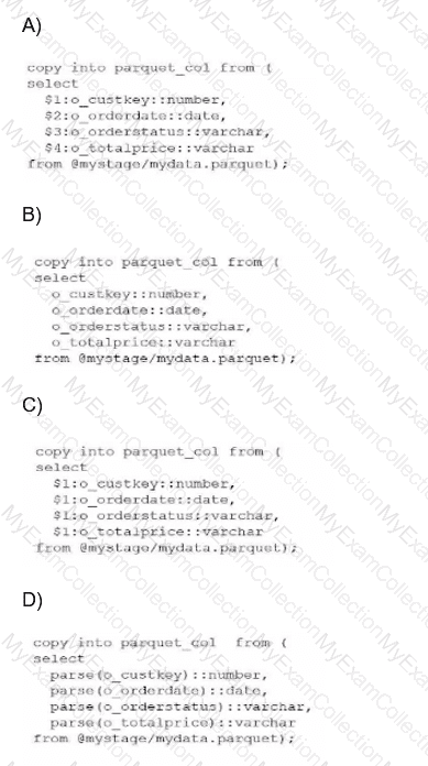
Question # 19
A Data Analyst has a Parquet file stored in an Amazon S3 staging area. Which query will copy the data from the staged Parquet file into separate columns in the target table?
A.
Option A
B.
Option B
C.
Option C
D.
Option D
Full Access
Answer:
C
Explanation:
In the Snowflake ecosystem, Parquet is treated as a semi-structured data format. When you stage a Parquet file, Snowflake does not automatically parse it into multiple columns like it might with a flat CSV file. Instead, the entire content of a single row or record is loaded into a single VARIANT column, which is referenced in SQL using the positional notation $1.
The fundamental mistake often made—and represented in Option A—is treating Parquet as a delimited format where $1, $2, and $3 refer to different columns. In Parquet ingestion, columns $2 and beyond will return NULL because the schema is contained within the object in $1.
To successfully "shred" or flatten this semi-structured data into a relational table with separate columns, an analyst must use path notation. This involves referencing the root object ($1), followed by a colon (:), and then the specific element key (e.g., $1:o_custkey). Furthermore, because the values extracted from a Variant are technically still Variants, they must be explicitly cast to the correct data type using the double-colon syntax (e.g., ::number, ::date) to ensure they land in the target table with the correct data types.
Evaluating the Options:
Option A is incorrect because it uses positional references ($2, $3, etc.) which are only valid for structured files like CSVs.
Option B is incorrect because it attempts to reference keys directly without the required stage variable ($1) and colon separator.
Option D is incorrect as it uses a non-standard parse() function that does not exist for this purpose in Snowflake SQL.
Option C is the 100% correct syntax. It correctly identifies that the Parquet data resides in $1, utilizes the colon to access internal keys, and applies the necessary type casting. This specific method is known as "Transformation During Ingestion" and is a core competency for any SnowPro Advanced Data Analyst.